As we mentioned in a previous blog post, A CG production can be represented as a graph structure. A movie is made of shots which are generated from scene files which are themselves made of elements linked by relationships. Nevertheless, when we store production data into a database, we tend to use a flat description of the data. And when it’s time to chose a database, the most common choice is to rely on relational databases.
Using a relational database is a good choice: it’s safe and does the job well. But, nowadays, a few database technologies propose to store your data directly formatted as graphs. Initially, they are mostly used to deal with social networks or banking use cases. But it’s no suprise that they caught the attention of many Technical Directors and Developers from CG studios. Because of the growing interest for graph databases, we decided to look closer at them.
The information of a graph will make you more agile. Graph storage allows to save the dependencies of all your assets and set the versions of the elements casted in a shot. And because stored graphs are directed, you can easily compute a sequence of operations to build or rebuild an element of the scene. Which means more reactivity when the director wants to try new things.
Now we have a good incentive to use graph databases, we are going to have a look at major open source graph databases available on the market.
Example use case
To explore these databases, we propose to implement the data graph of the props animation described in our previous article named CG production as a Graph. The approach will be to store the steps required to build the props and include it in a given shot.
The most common thing we want to do with graph is to obtain all the impacts of a change on a given element. To illustrate this, we will perform a query that retrieve the elements impacted by the change on the mesh of the props.
We’ll provide Python snippets to show how to use each database. Then we’ll run a quick benchmark. We will compare how long it takes to run 10 000 times our sample query on a i7–6700 CPU @ 3.40GHz . Note that this benchmark includes the Python client, we consider that you will only use your database through it. That’s why we include it in our measures.
Main databases
The main databases we will study are the following:
Cayley
Cayley is a graph database distributed by Google written in Go. It looks promising on many aspects (configurable backend, community driven) but currently the documentation is close to inexistant. Whatever, let’s see what we can do with.
First, download the binaries related to your platform, initialize the database and run the http server which will that allow us to perfoms queries. Database initialization doesn’t mean you have to give data, it’s just needed to create the database files../cayley init -db bolt -dbpath /tmp/testdb
./cayley http --dbpath=/tmp/testdb --host 0.0.0.0 --port 64210
You can notice here that another DB technology is involved (Bolt). It’s because Cayley is a layer above an existing database. You can either use traditional key value stores or relational database as backend.
Now let’s go with the Python client code. We want to store all our assets, scenes, shots and their relations. To achieve that, we need to install the Python driver:pip install pyley
Cayley is based on the concept of triplet. Everything is a vertex linked to another one: the triplet is made of three vertices: the two elements we want to link and the link vertex (kind of edge). You can add a label on each triplet, so in Cayley the term for this data structure is “quads”.
Unfortunately the Python client is not complete and does not support Quad creation. So we need to create our quads via requests, a standard Python HTTP client (Cayley provied a REST API):def create_quad(quad):
path = “http://localhost:64210/api/v1/write"
return requests.post(path, json=[quad])
Now let’s proceed to the quad creation:quads = [
{
“subject”: “props1-concept”,
“predicate”: “dependencyof”,
“object”: “props1-texture”
},
{
“subject”: “props1-concept”,
“predicate”: “dependencyof”,
“object”: “props1-mesh”
},
{
“subject”: “props1-texture”,
“predicate”: “dependencyof”,
“object”: “props1-model”
},
{
“subject”: “props1-mesh”,
“predicate”: “dependencyof”,
“object”: “props1-model”
},
{
“subject”: “props1-mesh”,
“predicate”: “dependencyof”,
“object”: “props1-rig”
},
{
“subject”: “props1-mesh”,
“predicate”: “dependencyof”,
“object”: “props1-keys”
}
{
“subject”: “props1-rig”,
“predicate”: “dependencyof”,
“object”: “props1-keys”
},
{
“subject”: “props1-model”,
“predicate”: “dependencyof”,
“object”: “shot1-image-sequence”
},
{
“subject”: “props1-keys”,
“predicate”: “dependencyof”,
“object”: “shot1-image-sequence”
}
]for quad in quads:
create_quad(quad)
That’s it. As you can see we already have stored all our data and set relation between them. If you create again similar quads, nothing will change and there will be no duplicates.
Now let’s perform our query about the impact of a rig change on the production:from pyley import CayleyClient, GraphObject
client = CayleyClient("http://localhost:64210", "v1")graph = GraphObject()
query = graph.V(“props1-mesh”)
.Out()
.All()
To get our desired data, we had to specify which vertex (here our texture) of which we want to study the impact of. Then we just asked the outer the vertex of wich the texture is element of. We can chain the call depending on the depth of the impact we want to study. A recursive traversal is available but the Python client doesn’t implement it yet. Finally we made our performance tests. It took 50 seconds to run ten thousands time this query.
The visualization UI doesn’t work well and is not very intuitive to use. Which is sad because Neo4j and Arango have working UIs that allow to display your graph.
Cayley is a very simple database. With a single concept, the quad representation, it allows to represent our data. Querying is very easy too and based on standard graph query language such as Gremlin (you can chose your favorite query language). Unfortunately the project is still poorly documented and the Python client is uncomplete. That’s why despite its clean and simple design we cannot recommend to use Cayley in production.
Neo4j
Neo4j is the most mature solution of all. The enterprise behind it offers compelling entreprise solution for support and extra features (monitoring, backup, improved querying…). That’s a big advantage if you need to feel very safe due to hard contracts with your clients. But to start with it, we reommend using the community edition. This is this version that we’ll cover in this article.
Because we are just experimenting, we are going to use the official Docker to play with Neo4j:
docker run \ --publish=7474:7474 --publish=7687:7687 \ --volume=$HOME/neo4j/data:/data \ neo4jNow we can install the Python driver:pip install neo4j-driver
First things first, let’s initialize the connection with the database and the query session. At first connection they will ask you to set a password, you can do it through the last line of the snippet below:from neo4j.v1 import GraphDatabase, basic_authdriver = GraphDatabase.driver(
"bolt://localhost:7687",
auth=basic_auth("neo4j", "tests")
)
session = driver.session()
# session.run("CALL dbms.changePassword('tests')")
Then let’s add helpers to create asset nodes, shot nodes and relation edges. The python client does not provide a strong API, it justs allow to perform requests directly with the in-house language of Neo4j named Cypher. There is CREATE command but we’ll use MERGE because it acts as CREATE if not exists:def create_asset(name):
session.run(
"MERGE (a:Asset { name: $name })",
name=name
)def create_shot(name):
session.run(
"MERGE (a:Shot { name: $name })",
name=name
)def create_relation(asset1, asset2):
session.run(
"MATCH (a:Asset { name: $asset1 }), (b:Asset { name: $asset2 })"
"MERGE (a)-[r:ELEMENT_OF]->(b)",
asset1=asset1, asset2=asset2
)def create_casting(asset, shot):
session.run(
"MATCH (a:Asset { name: $asset }), (b:Shot { name: $shot })"
"MERGE (a)-[r:CASTED_IN]->(b)",
asset=asset, shot=shot
)
As you can see the syntax is easy to read and learn. We can add as many fields we want on a single node.
Now we have our functions, let’s populate our graph:create_asset("Props 1 concept")
create_asset("Props 1 mesh")
create_asset("Props 1 texture")
create_asset("Props 1 rig")
create_asset("Props 1 model")
create_asset("Props 1 keys")
create_shot("Shot 1")create_relation("Props 1 concept", "Props 1 texture")
create_relation("Props 1 concept", "Props 1 mesh")
create_relation("Props 1 mesh", "Props 1 model")
create_relation("Props 1 texture", "Props 1 model")
create_relation("Props 1 mesh", "Props 1 rig")
create_relation("Props 1 mesh", "Props 1 keys")
create_relation("Props 1 rig", "Props 1 keys")create_casting("Props 1 model", "Shot 1")
create_casting("Props 1 keys", "Shot 1")
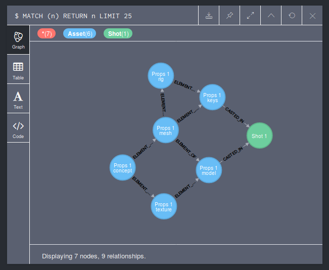
Now we can take advantage of the expressive query language to perform our traversal. Note the star inside the arrow. It means that will traverse all nodes until there is no more out connections.result = session.run(
"MATCH (:Asset { name: 'Props 1 mesh' })-[*]->(out)"
"RETURN out.name as name"
)for record in result:
print("%s" % record["name"])session.close()
We’re done! Result records are easy to display and analyze. They are Python dicts containing the fields specified at creation. Running ten thousand times our request lasted 3.5 seconds (it drops to 17 seconds if you open/close the session each time).
Overall, Neo4j is full featured and does the job well and it’s fast compared to others. Its strong query language and its many features will allow to perform the most common use cases you will have with your graph. The official Python client is a bit thin, but the community provides an interesting alternative with a client built like an ORM. Last but not least, the database is here since a long time and the entreprise behind it is very active. So, it makes Neo4j the safer choice of this review.
NB: here is a real life feedback about Neo4j.
With ArangoDB
ArangoDB is a versatile database that allows document storage and graph storage all along. Recently, it have gained in popularity, it’s the reason why we included it to the test. It comes with handful features like easy deployment on a cloud infrastructure and helpers to build REST API. But for this article we’ll focus on the graph storage and its query system.
Let’s code! To make our testing we need first an Arango instance up and running. Let’s use Docker again to spawn it:docker run -p 8529:8529 -e ARANGO_ROOT_PASSWORD=openSesame arangodb/arangodb:3.2.1
Then we install the Python client:pip install python-arango
Now we can write our Python script, the first step will be to initialize our database:from arango.client import ArangoClientclient = ArangoClient(username='root', password='openSesame')
db = client.create_database('cgproduction')
As you can see the database creation is very straightforward. The only problem is that it raises an exception if the database already exists. It means that if you want to achieve idempotence with your script, you will have to write your own “get or create” method. It’s the same for every creation we’ll do in the following. Be prepared to augment this Python driver.
The next step is to define our graph and configure the collections that will store vertices and edges information:dependencies = db.create_graph('dependencies')shots = dependencies.create_vertex_collection('shots')
assets = dependencies.create_vertex_collection('assets')casting = dependencies.create_edge_definition(
name='casting',
from_collections=['assets'],
to_collections=['shots']
)
elements = dependencies.create_edge_definition(
name='element',
from_collections=['assets'],
to_collections=['assets']
)
Arango graph storage is based on its own document storage system. Each vertex is stored as a json entry in a collection. Edges are a little bit different. They are stored in a similar fashion, but the collection definition requires more information: the inner vertex collection and the outer one. Edges are always directed.
Now we have our database properly configured, we can add our data:# Insert vertices
assets.insert(
{'_key': 'props1-concept', 'name': 'Props 1 Concept'})
assets.insert(
{'_key': 'props1-texture', 'name': 'Props 1 Texture'})
assets.insert(
{'_key': 'props1-mesh', 'name': 'Props 1 Mesh'})
assets.insert({'_key': 'props1-rig', 'name': 'Props 1 Rig'})
assets.insert({'_key': 'props1-model', 'name': 'Props 1 Model'})
assets.insert({'_key': 'props1-keys', 'name': 'Props 1 Keys'})
shots.insert(
{'_key': 'shot1-image-sequence',
'name': 'Shot 1 Image sequence'})# Insert edges
elements.insert(
{'_from': 'assets/props1-concept',
'_to': 'assets/props1-texture'})
elements.insert(
{'_from': 'assets/props1-concept',
'_to': 'assets/props1-mesh'})
elements.insert(
{'_from': 'assets/props1-texture',
'_to': 'assets/props1-model'})
elements.insert(
{'_from': 'assets/props1-mesh',
'_to': 'assets/props1-rig'})
elements.insert(
{'_from': 'assets/props1-mesh',
'_to': 'assets/props1-model'})
elements.insert(
{'_from': 'assets/props1-mesh',
'_to': 'assets/props1-keys'})
elements.insert(
{'_from': 'assets/props1-rig',
'_to': 'assets/props1-keys'})
casting.insert(
{'_from': 'assets/props1-model',
'_to': 'shots/shot1-image-sequence'})
casting.insert(
{'_from': 'assets/props1-keys',
'_to': 'shots/shot1-image-sequence'})
Once our data properly imported, we can proceed to our query:traversal_results = dependencies.traverse(
start_vertex=’assets/props1-mesh’,
direction=’outbound’
)for result in traversal_results[“vertices”]:
print(result[“name”])
With this simple request we get all our impact of a modification of the props 1 mesh. The result is easy to analyze and the query is configurable (for instance you can chose between a depth first traversal and a breath first traversal).
Arango provides a traversal object that allows you to build particular path. Some helpers are available too, like shortest path finding or path length retrieval. It should cover most of your needs in term of graph querying.
Last but not least, you can visualize your graph in the Arango web UI:
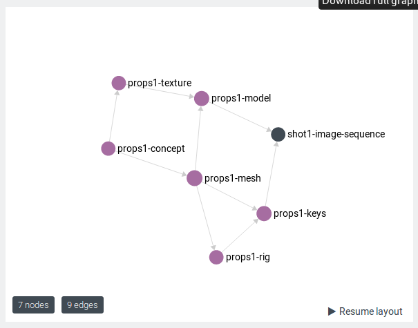
Overall, the ArangoDB and Python client are simple to understand and well documented. It provides many helpers to play with our graph and the visualization tools makes things even easier. But it looks slower than neo4j. Running 10 000 times our query took 26s. Despite these results, it’s still our favorite database of this test. Arango is very developer-friendly. It is the best choice to experiment quickly with graph databases. And because the company behind looks very active, it seems to be a safe choice for a production usage too.
OrientDB
OrientDB is here for a while now (since 2010). But because of the very bad feedback about it (see comments too), we decided to not cover this database in this article. It’s too risky to use it in a CG production environment.
Alternatives
There are still alternatives. By playing with traditional database, you can have similar features as with graph database. One option is to use Postgres with its recursive joins. It will allow you to cover simple use cases of graph traversal.
Another option, which looks great if you want to be able to do fuzzy searches, is to use Elastic Search and store all vertices and edges as JSON documents (similar approach as ArangoDB). Read this full article to have more information about the subject.
Visualisation
Having graph data is great but you may want to build tools that shows your data at some point (and outside of the built-in UIs).
There are two good libraries for Qt that allows to build graph easily:
- ZodiacGraph: a powerful C++ library which is fast and flexible.
- Nodz: a Python library easy to use.
Another option is to use Javascript libraries for in-browser or Electron applications. Here are some:
- SigmaJS: fast and well documented library
- Cytoscape: versatile and robust.
- d3.js: harder to use but limitless.
To conclude
From our study, it looks like ArangoDB is the most user friendly database and its document storage aspect will make your production data management easier. But it’s still a young DB. If you need speed or if there is a lot of money at stake and if you are looking for a safer choice go for Neo4j, which does the job well and looks more robust. Finally Cayley looks good on many aspects has a great design and could be the best choice to complement an already existing relational database, but is still too undocumented and young to be used in production. So, to sum up: try ArangoDB first!
The question about what problems solve graph representation and storage for pipeline TDs remain. The main use case for us is to generate easily the sequence of actions needed to rebuild a shot when a change occurs. The other one is to provide easily a representation of the production on which people can discuss.
We hope you enjoy this article. We are still very new to graph databases. We would be glad to know what you think about it and read your production experience with these technologies: comments are welcome!
This blog is dedicated to CG pipeline and production management. If you are interested in graph databases for CG productions, you will probably enjoy all our articles. Read our first blog post to know more about us!